Real Data Example: PhysioNet Challenge 2019 Data in the EHRData Format#
This tutorial demonstrates how EHRData structures real-world longitudinal clinical data using the PhysioNet Challenge 2019 (Early Prediction of Sepsis from Clinical Data) dataset.
Note
It is helpful to check out the Getting started with EHRData to learn the basics of EHRData before diving into this tutorial.
The PhysioNet Challenge 2019 dataset contains ICU patient data. It was designed to encourage the development of algorithms for early detection of sepsis using physiological data [RJJ+20] [GAG+00].
Dataset Overview#
The dataset includes:
40,336 ICU patients from two hospital systems
35 time-dependent clinical variables (vitals, lab values, etc.)
5 static features: Age, Gender, Unit1, Unit2, HospAdmTime
Hourly measurements with variable-length stays
Outcome:
SepsisLabel- binary indicator of sepsis onset
Key clinical variables include:
Vital signs: HR, O2Sat, Temp, SBP, MAP, DBP, Resp
Laboratory values: Glucose, Lactate, Creatinine, Bilirubin, WBC, Platelets
Blood gas: pH, PaCO2, SaO2, BaseExcess, HCO3, FiO2
Let’s explore how EHRData organizes this complex data structure!
Loading the Dataset#
The ehrdata package provides multiple datasets out-of-the-box, and PhysioNet 2019 is one of them.
See physionet2019() for more details about how the dataset is loaded.
import ehrdata as ed
import numpy as np
import matplotlib.pyplot as plt
This downloads the data if needed and processes it into an EHRData object:
edata = ed.dt.physionet2019(layer="tem_data", n_samples=1000)
edata
View of EHRData object with n_obs × n_vars × n_t = 1000 × 35 × 48
    obs: 'Age', 'Gender', 'Unit1', 'Unit2', 'HospAdmTime', 'training_Set'
    var: 'Parameter'
    tem: '0', '1', '2', '3', '4', '5', '6', '7', '8', '9', '10', '11', '12', '13', '14', '15', '16', '17', '18', '19', '20', '21', '22', '23', '24', '25', '26', '27', '28', '29', '30', '31', '32', '33', '34', '35', '36', '37', '38', '39', '40', '41', '42', '43', '44', '45', '46', '47'
    layers: 'tem_data'
    shape of .tem_data: (1000, 35, 48)
Note
The first time you run this, it will download ~40MB of data. Subsequent runs will use the cached version.
We use n_samples=1000 to speed up the tutorial - remove this parameter to load the full dataset of 40,336 patients.
Reminder: the EHRData Structure#
![]()
An EHRData object organizes data across three dimensions:
n_obs: Number of observations (patients/ICU stays)n_vars: Number of variables (clinical parameters)n_tem: Number of temporal measurements (time points)
Let’s explore its key components with PhysioNet Challenge 2019 data!
The .layers Attribute: Time Series Data#
The .layers attribute contains the 3D tensor of shape (n_obs, n_vars, n_tem) with all time series measurements:
print(f"Shape of layers: {edata.layers['tem_data'].shape}")
print(f"Data type: {edata.layers['tem_data'].dtype}")
print("\nThis represents:")
print(f"  - {edata.n_obs} patients")
print(f"  - {edata.n_vars} clinical variables")
print(f"  - {edata.n_t} time intervals (hours)")
Shape of layers: (1000, 35, 48)
Data type: float64

This represents:
  - 1000 patients
  - 35 clinical variables
  - 48 time intervals (hours)
The .obs Attribute: Static Patient Metadata#
The .obs DataFrame contains static information for each patient:
edata.obs.head()
| Age | Gender | Unit1 | Unit2 | HospAdmTime | training_Set | |
|---|---|---|---|---|---|---|
| RecordID | ||||||
| p000012 | 81.64 | 1.0 | 1.0 | 0.0 | -0.03 | training_setA |
| p000108 | 88.90 | 0.0 | NaN | NaN | -76.49 | training_setA |
| p000142 | 55.89 | 1.0 | 1.0 | 0.0 | -0.02 | training_setA |
| p000197 | 22.94 | 1.0 | NaN | NaN | -14.35 | training_setA |
| p000211 | 70.50 | 1.0 | 1.0 | 0.0 | -67.75 | training_setA |
The .obs table here includes:
Static variables: Age, Gender, Unit1 (medical ICU), Unit2 (surgical ICU), HospAdmTime (hours before ICU), training_Set (dataset provided split)
Note that the index is the RecordID - a unique identifier for each patient.
The .var Attribute: Variable Metadata#
The .var DataFrame can contains information about each clinical variable being measured. Here, this is just the parameter name; it can be expanded to include e.g. Units, or alternative names.
print(f"Number of variables: {edata.n_vars}\n")
print("Clinical variables:")
edata.var
Number of variables: 35

Clinical variables:
| Parameter | |
|---|---|
| Parameter | |
| AST | AST |
| Alkalinephos | Alkalinephos |
| BUN | BUN |
| BaseExcess | BaseExcess |
| Bilirubin_direct | Bilirubin_direct |
| Bilirubin_total | Bilirubin_total |
| Calcium | Calcium |
| Chloride | Chloride |
| Creatinine | Creatinine |
| DBP | DBP |
| EtCO2 | EtCO2 |
| FiO2 | FiO2 |
| Fibrinogen | Fibrinogen |
| Glucose | Glucose |
| HCO3 | HCO3 |
| HR | HR |
| Hct | Hct |
| Hgb | Hgb |
| Lactate | Lactate |
| MAP | MAP |
| Magnesium | Magnesium |
| O2Sat | O2Sat |
| PTT | PTT |
| PaCO2 | PaCO2 |
| Phosphate | Phosphate |
| Platelets | Platelets |
| Potassium | Potassium |
| Resp | Resp |
| SBP | SBP |
| SaO2 | SaO2 |
| SepsisLabel | SepsisLabel |
| Temp | Temp |
| TroponinI | TroponinI |
| WBC | WBC |
| pH | pH |
The .tem Attribute: Temporal Information#
The .tem DataFrame contains information about the time intervals:
print(f"Number of time intervals: {edata.n_t}\n")
edata.tem.head(10)
Number of time intervals: 48
| interval_start_offset | interval_end_offset | |
|---|---|---|
| interval_step | ||
| 0 | 0 days 00:00:00 | 0 days 01:00:00 |
| 1 | 0 days 01:00:00 | 0 days 02:00:00 |
| 2 | 0 days 02:00:00 | 0 days 03:00:00 |
| 3 | 0 days 03:00:00 | 0 days 04:00:00 |
| 4 | 0 days 04:00:00 | 0 days 05:00:00 |
| 5 | 0 days 05:00:00 | 0 days 06:00:00 |
| 6 | 0 days 06:00:00 | 0 days 07:00:00 |
| 7 | 0 days 07:00:00 | 0 days 08:00:00 |
| 8 | 0 days 08:00:00 | 0 days 09:00:00 |
| 9 | 0 days 09:00:00 | 0 days 10:00:00 |
Exploring Individual Patients#
Let’s visualize the time series data for a single patient to understand the temporal structure:
# Select the first patient
patient_idx = 0
patient_id = edata.obs.index[patient_idx]
patient_data = edata[patient_idx, :, :]

print(f"Patient ID: {patient_id}")
print(f"Age: {edata.obs.loc[patient_id, 'Age']:.1f} years")
print(f"Gender: {'Male' if edata.obs.loc[patient_id, 'Gender'] == 1 else 'Female'}")
print(f"Data shape: {patient_data.layers['tem_data'].shape}")
Patient ID: p000012
Age: 81.6 years
Gender: Male
Data shape: (1, 35, 48)
# Select a few vital signs to visualize
vital_signs = ["HR", "O2Sat", "Temp", "SBP", "Resp"]
var_indices = [list(edata.var_names).index(v) for v in vital_signs if v in edata.var_names]

fig, axes = plt.subplots(len(var_indices), 1, figsize=(12, 2.5 * len(var_indices)), sharex=True)

for ax, var_idx in zip(axes, var_indices, strict=False):
    var_name = edata.var_names[var_idx]
    values = edata.layers["tem_data"][patient_idx, var_idx, :]
    time_points = np.arange(len(values))

    # Plot only non-NaN values
    mask = ~np.isnan(values)
    ax.plot(time_points[mask], values[mask], "o-", markersize=4, label=var_name)
    ax.set_ylabel(var_name)
    ax.legend(loc="upper right")
    ax.grid(visible=True, alpha=0.3)

axes[-1].set_xlabel("Hours since ICU admission")
fig.suptitle(f"Patient {patient_id} - Vital Signs Over Time", fontsize=14)
plt.tight_layout()
plt.show()
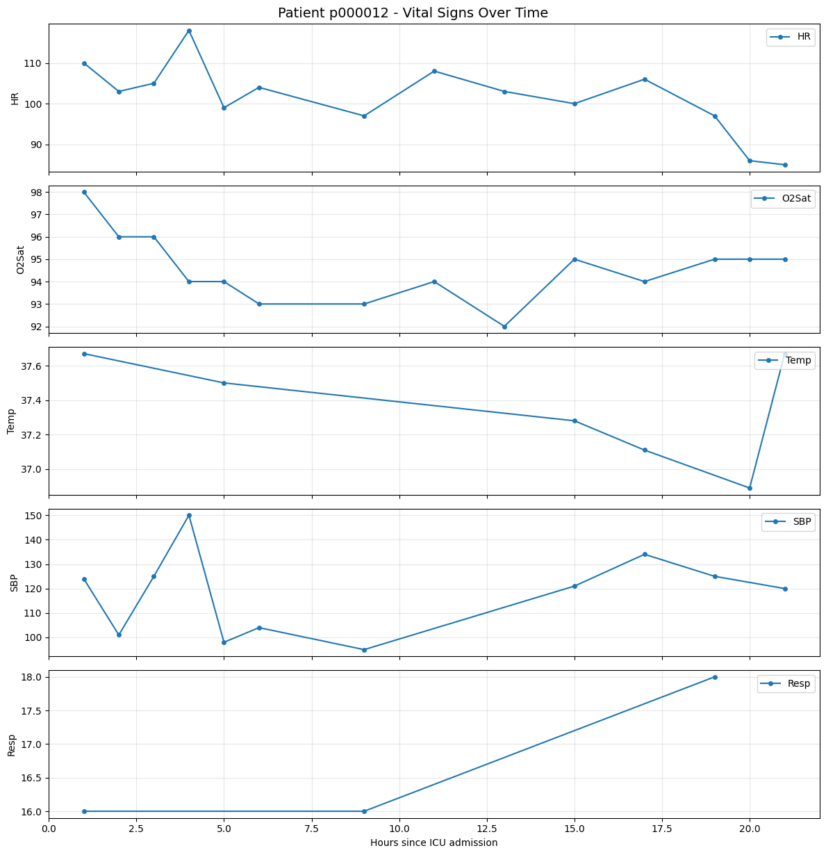
These plots illustrate how variables such as HR develop over time for an individual patient.
The good news: You don’t need to write a lot of code for such visualizations anymore!
ehrapy has many utility functions for processing and vizualizing data in the EHRData format - for a fancy version of this plot here, available interactively powered by bokeh, see for instance timeseries()
Subsetting and Filtering#
EHRData supports powerful subsetting operations similar to numpy arrays:
# Get patients who developed sepsis (SepsisLabel = 1 at any time point)
sepsis_var_idx = list(edata.var_names).index("SepsisLabel")
sepsis_data = edata.layers["tem_data"][:, sepsis_var_idx, :]

# A patient has sepsis if SepsisLabel is 1 at any time point
has_sepsis = np.nanmax(sepsis_data, axis=1) == 1

print(f"Patients with sepsis: {has_sepsis.sum()} out of {len(has_sepsis)}")
print(f"Sepsis rate: {has_sepsis.mean() * 100:.1f}%")

# Subset to sepsis patients
sepsis_patients = edata[has_sepsis, :, :]
print(
    f"\nSubsetted EHRData shape: {sepsis_patients.n_obs} patients × {sepsis_patients.n_vars} variables × {sepsis_patients.n_t} hours"
)
Patients with sepsis: 48 out of 1000
Sepsis rate: 4.8%

Subsetted EHRData shape: 48 patients × 35 variables × 48 hours
Choosing different time intervals#
Depending on the question at hand, different time intervals are of interest.
For the physionet2019(), in the intensive care unit setting, the observations of patient data happen within minutes to hours, and usually only for a few days.
For observational health data, the observations happen rather across weeks or months, and span for many years.
The physionet2019() function provides arguments to specify more about the time intervals. We can for instance load the data with a different time resolution (2-hour intervals, 24 intervals total)
edata_2h = ed.dt.physionet2019(
    layer="tem_data", n_samples=1000, interval_length_number=2, interval_length_unit="h", num_intervals=24
)
print(f"Shape with 2-hour intervals: {edata_2h.layers['tem_data'].shape}")
print(f"Now we have {edata_2h.n_t} time points instead of {edata.n_t}")
Shape with 2-hour intervals: (1000, 35, 24)
Now we have 24 time points instead of 48
If we plot this again, we can see the data is less fine-grained now:
# Visualize the same patient with 2-hour intervals
fig, axes = plt.subplots(len(var_indices), 1, figsize=(12, 2.5 * len(var_indices)), sharex=True)

for ax, var_idx in zip(axes, var_indices, strict=False):
    var_name = edata_2h.var_names[var_idx]
    values = edata_2h.layers["tem_data"][patient_idx, var_idx, :]
    time_points = np.arange(len(values)) * 2  # 2-hour intervals

    mask = ~np.isnan(values)
    ax.plot(time_points[mask], values[mask], "o-", markersize=4, label=var_name)
    ax.set_ylabel(var_name)
    ax.legend(loc="upper right")
    ax.grid(visible=True, alpha=0.3)

axes[-1].set_xlabel("Hours since ICU admission")
fig.suptitle(f"Patient {patient_id} - Vital Signs (2-hour intervals)", fontsize=14)
plt.tight_layout()
plt.show()

Next Tutorial#
Continue with OMOP Introduction to learn how to read any dataset in the OMOP Common Data Model.
Further Resources#
PhysioNet 2019 Challenge - The original challenge and dataset description
Sepsis-3 Definitions - Clinical definitions of sepsis